Getting the World Record in HATETRIS
Tetris That Hates You
 StickManStickMan #611, by Sam Hughes.
HATETRIS is a version of Tetris written in 2010 by programmer and sci-fi author Sam Hughes. According to his initial description of the game:
This is bad Tetris. It’s hateful Tetris. It’s Tetris according to the evil AI from “I Have No Mouth And I Must Scream”.
(And if you aren’t familiar with Tetris at all, and don’t know the rules or pieces, we recommend trying out the original game for yourself; Wikipedia has an article about how Tetris in particular can consume your life and enter your very dreams, but we’re sure you’ll be fine.)
The hatred comes from the way pieces are selected. In most variants of Tetris, the piece selection is pseudorandom, with methods ranging from independently random selection to the more recent Bag Random Generator. In almost every variant that isn’t truly random, the changes to randomness are done to make the player less likely to get two pieces of the same type in a row, or to go too long without seeing a given piece.
HATETRIS selects pieces in almost precisely the opposite manner, with a one-move lookahead min-max algorithm:
- First, check every possible position for all seven pieces.
- Second, among those positions, examine how ‘good’ each of these moves is for the player, by measuring how high the highest block in the well is.
- Third, select the piece which has the worst best-case scenario for the player. If there is a tie, break the tie in the piece order
S, Z, O, I, L, J, T.
There’s no randomness involved: the first, second, and third pieces you get upon starting the game will always be the S piece, and so will most of the others throughout the game. There’s no next piece window, since the next piece isn’t decided until you finish your move. There’s no possibility at all of getting four lines at once with a well-placed I piece, since the game will never under any circumstances give you an I-piece that you could use to clear four lines. And, in general, if you’ve set up to clear a line and there’s any piece at all which denies you that line for at least a turn, that’s the piece you’re going to get.
It’s a common experience for players to try the game for the first time with a strategy perfectly sound for normal Tetris and score no points at all, simply because normal Tetris strategy amounts to setting up good situations and then waiting for the odds to be in your favor. With a deterministic algorithm like this one, the odds will never be in your favor.
High Scores
The flip side of determinism is predictability. Because the algorithm will always return the same move given the same history of moves, it’s possible to plan ahead and come up with complex strategies that one could never use in a non-deterministic game - and it’s possible to share results. The first few records (Mr. Hughes’ initial game of 5 points, and commenter JeremyBowers’ and Kazanir’s claims at seven points) were lost to history, but once replay functionality was added the day after release, the comment section became a leaderboard, and anyone could take an existing replay and copy the moves to try to improve on the same strategy.
Commenter Atypical posted the first replay, an eleven-point run, and over the next month, the high score was pushed to 17, 20, 22, 28, and finally 30, all using the same opening sequence of moves to create wells where every piece can be used to clear a line, four or five times in a row. This sequence of moves was so successful, in fact, that every world record run for ten years after its discovery used it. The Atypical strategy consisted of stackingS-pieces to the left of the well, clearing as many lines as possible, building a flat ‘ceiling’ on top of the pieces currently in the well, and then effectively starting from scratch on top of that ceiling. By the time of the 30-point runs, the Atypical strategy was so successful that it was even done a third time, near the end of the game. So far as we know, there isn’t a term for this, so we call this a pseudoloop; you’re not getting back to the same well you had before, but you’re doing the same pattern over and over again.
This score of 30 points, set a month after release by the Japanese Slashdot poster Deasuke, held for the next seven years. When we started playing the game in 2013, we assumed that 30 points was as high as humans would ever get, and was probably as high as the game’s mechanics would allow. But around 2017, we started tinkering a bit with machine learning, and the question naturally came up: could a program be written to beat HATETRIS? We floated around a few ideas - including what would have been a very primitive version of a Monte-Carlo tree search - but never got around to implementation, even after commenter chromeyhex eked out another point a few months later and proved that 30 was not the maximum after all. It wasn’t until June of 2021, when commenter knewjade optimized the final few moves of the existing high score to get a score of 32, and then 34 points two days later, that we decided to start coding in earnest.
And then, a week after that, knewjade got 41 points…and did so with a somewhat different opening sequence than the one which had been used and improved upon for ten years. And a week later, he pushed it to 45. The Rust emulator was working by that point and the program could play around a hundred random games per second…but that was about all it could do, and we weren’t even close to using any machine learning yet. We breathed a slow sigh of relief as weeks went by and our own project made progress with no new world records being set, until knewjade in late August of 2021 posted a high score completely unlike any game known to exist for HATETRIS, totalling 66 points.
This game is beautiful. Pieces set up in clearly unclearable positions turn out to be vital to clearing a line ten moves later, and it isn’t until fifteen points in that knewjade is forced to allow even a single hole higher than the first line. There are no pseudoloops - the shape of the well is constantly changing, and the well is quite frequently piled up almost to the top of the well to then clear multiple lines one after the next. By this point, knewjade had posted an explanation of the code he used to find these new high scores (and this explanation will be key to our success, later), but even without the explanation, it was very clear that there was machine search involved somewhere. The game was simply too novel, discovered too quickly, and optimized too well, to have been done by a human being unaided. So it was possible for a machine to learn HATETRIS - we just had to learn how to teach it.

Choosing a Language
For starting the project, our shortlist came down to three languages: Mathematica, python, and Rust. Each had various pros and cons:
- Mathematica: Pros: huge amount of personal experience, huge number of useful built-in functions for machine learning and general analysis, easy to make visualizations or monitor in a dynamic way. Cons: slower than molasses in January.
- Python: Pros: Lots of good built-in machine learning APIs, like Tensorflow, Keras, and PyTorch. Faster than Mathematica. Cons: Still slower than compiled languages.
- Rust: Pros: Extremely fast. Cons: Not much in the way of built-in machine learning tools.
Everything ultimately came down to speed; no matter what the plan, or what variant of machine learning we were going to do, we’d need vast quantities of data, and we’d need to get that data with a single mid-range desktop computer. And calculating the legal HATETRIS moves was going to take time; the initial implementation of the game in Javascript mentioned that the algorithm is “quite time-consuming to execute, so please forgive me if your browser chugs a little after locking each piece”. So, to get as many games and as much data as we could, we’d need every advantage, starting with the fastest language we personally knew.
As a point of reference, the first speed test we did was playing random games with an unoptimized emulator in Mathematica, and the same unoptimized emulator in Rust. Mathematica took 4.3 seconds per game on average, and Rust took 0.035 seconds per game on average. This was such a big difference that we deemed that all of the hassle and aggravation of negotiating with Rust’s borrow checker would be worth it.
The Story So Far
When we first started on this project, we had a very clear idea of what we thought a winning strategy would be: A Monte Carlo simulation, powered by Machine Learning! Just like they do in AlphaGo and the more generalized AlphaZero. Surely someone had already written an implementation and all we had to do was write an emulator, hook it up to a nebulous AlphaZero implementation and emerge with a world record. How long could it take? Two weeks?
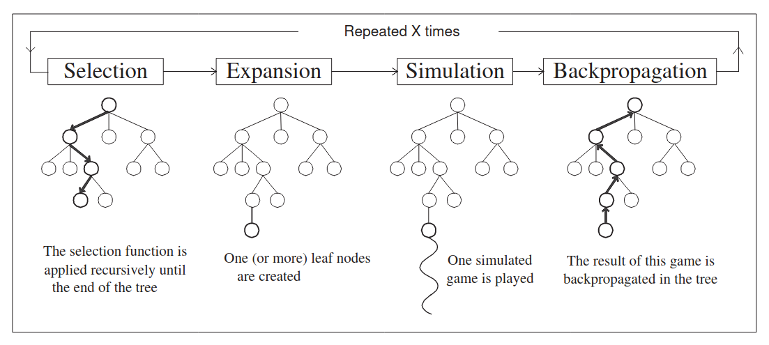
MCTS
MCTS (Monte-Carlo Tree Search) is a well-trod path in gameplay simulations. Without getting into details, since the methodology behind MCTS is much better explained elsewhere, the core conceit is to make each move in a game into a tree-like structure and then explore the tree.
Implementing a tree structure for HATETRIS positions was achievable. It was only after the initial tree implementation that we considered that there would be a lot of repeated wells: after all, in this game you can reach the same position in a number of different ways. A lot of deliberation and a re-factored codebase later, we opted for a directed acyclic graph (DAG) instead, taking identical positions and merging them into the same entry in a graph, rather than making them distinct entries on a tree. This complicated things significantly, but reduced our memory needs by an order of magnitude, at least. Refactoring from tree searches to DAG searches was more work than we’d expected to put in to the project, but was yielding promising results. An early depth first search got us scores of up to 14, with a simple greedy search looking for easy scores. At the time, the record was sitting at 34, so we felt very confident that we were on the right track.
It was sobering to realize, also, that “Graph vs Tree” in MCTS was in fact a discussion happening in professional circles. For example, this paper, which we read and didn’t fully comprehend, had a very succinct explanation of how DAGs were different from trees, and why it mattered:

We highlight that we fully failed to understand these, because there’s two things we learned from this:
- Reading the academic papers is important, because sometimes experts have the same problems you do.
- You don’t have to understand the whole paper (or most of the paper) to derive useful insights. Sometimes looking at the pictures is enough.
By this point we had a working emulator and a directed acyclic graph, and were ready to get rolling.
MCTS + AlphaZero
As it turns out, there is no “AlphaZero generic game engine that magically gets you world records” in Rust. There might be one in Python. Regardless, we could not just plug our MCTS to a magic library and hope for things to happen. Oh no. Instead, we had to build a monstrosity of layers using tch, a Rust-Pytorch-C binding library to make a model to train. The details of this are interesting, but not ultra-relevant to our world record run. We plan on writing a more detailed post-mortem after this blog where we dissect that at length. The main takeaways:
- Training a model took a long time, in the order of weeks.
- Mutating hyperparameters to improve results was difficult with long runtimes.
- We only had a few tens of thousands of games to train on, which made the learning extremely poor.
- Weeks and weeks of iteration produced worse and worse models, some overtrained, others just terrible.
- We were likely doing several things that would get us summarily exiled by real machine learning engineers.
Now, we are going to intentionally gloss over the giant, annoying mess that was multithreading our MCTS, a tangled web of mutexes, arc(mutexes) and locking paths that we still haven’t cleaned the bugs out of. We even had to make our own branch of tch to support mutexing the learning network. In summary: We tried multithreading. It improved performance. But our models were… awful, taking two full months to get back to where the simple, greedy MCTS search had gotten us in a couple of days. And they showed no signs of ever improving.
As a desperate last maneuver, we looked to knewjade’s new shiny record (66, at this point in time). Using knewjade’s heuristic, we generated ten thousand more MCTS games (the best of which scored 20 points), fed them to the model, and let it cook for two weeks. The resulting model was somehow worse than our training data, scoring at most 17. Which meant our poor model was just never going to rise above its training data. Not with the meager resources we could provide it.
AlphaHATETRIS was officially dead.
The Emulator
So, with AlphaHATETRIS dead, what did we have to work with? Well for starters, we’d written a pretty darn good emulator. Our best version is still not the best version that exists, but it worked well for our needs. How does this emulator work, anyway?
Well, Well, Well
Some quick terminology, since we’ll be using the word “well” and “move” until they lose all meaning:
- A well is the
20 x 10area in which the game is played, and any blocks currently in it. In general, when we talk about a well, you can think of it as a snapshot of a game in progress. - A piece is the four-block shape being maneuvered around in the well. When the piece cannot move down any further, it merges with the well and stops moving. This generates a new well.
- A position refers to a legal placement of a piece within the well, be it terminal or not.
- A terminal position is a piece that has reached a position where it can no longer descend, that is, it is going to become part of the well, exactly where it is. It’s terminal because once this piece is placed, we have created a new well.
- A move is a placement of a piece within a well, such that it is terminal, and generates a new well. We do not consider non-terminal motion inside the well to be a ‘move’.
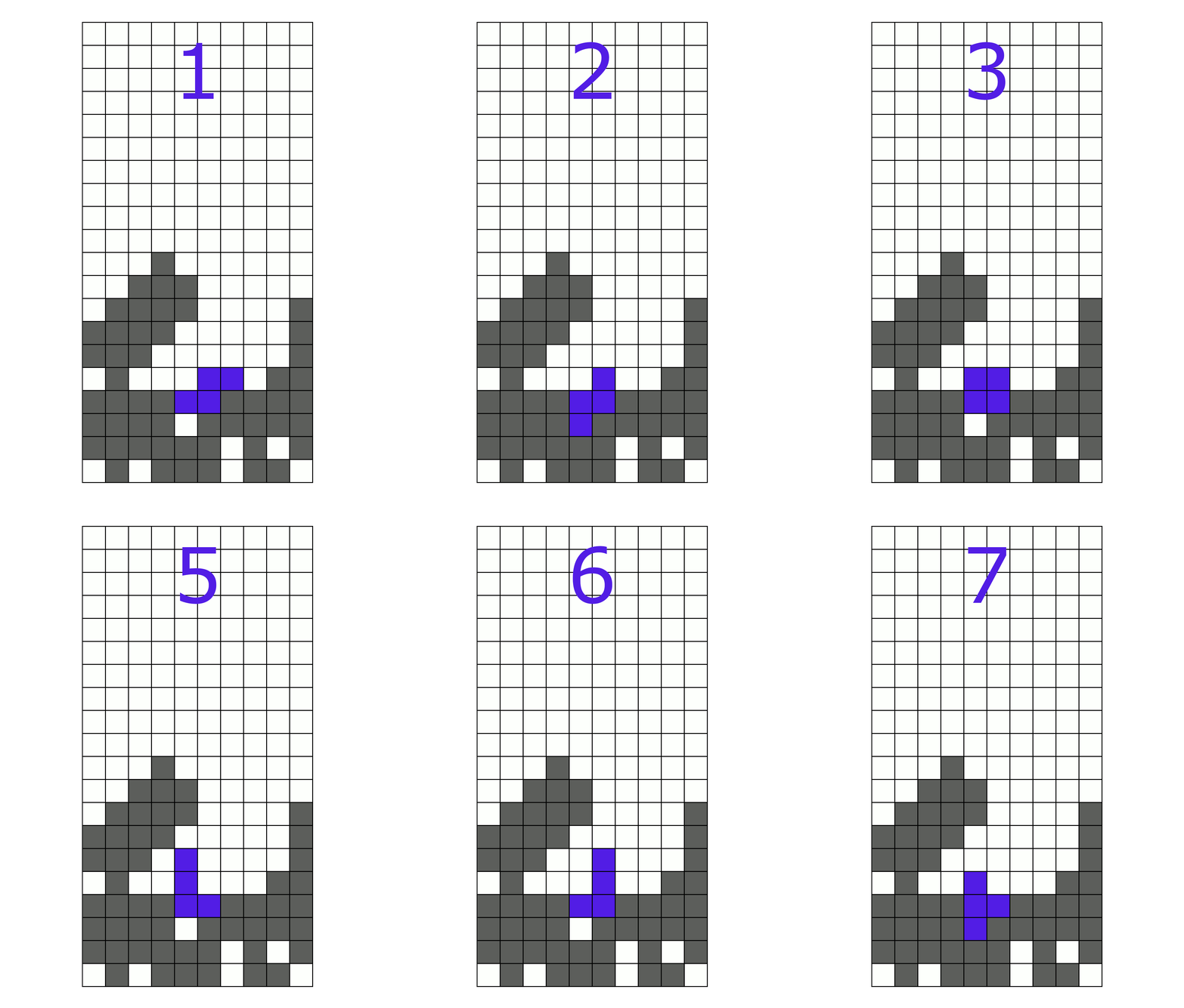
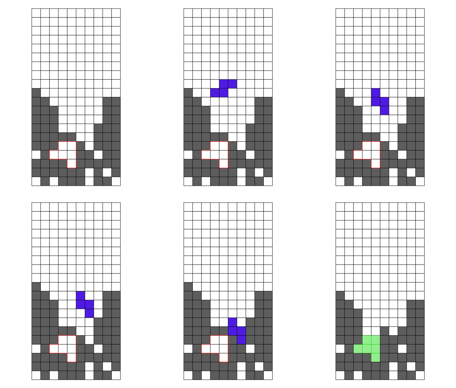
 (Left: A piece, in blue, at the beginning of its move. Center: a piece at the end of its move, in a terminal position. Right: a piece, in blue, at the beginning of the next move. The previous piece has merged with the rest of the well, indicated by the grey squares.)
Basic State Management
Our first draft was the obvious approach, considering every possible position by every possible piece, and repeating until there are no new positions left.
Move generation in this context, refers to only generating the moves for a specific well. That is, each time you get a piece, what are the places the piece could go?
Our initial version of the emulator took a well, and considered all the possible positions for the piece inside the well:
- First, take the initial position, and calculate the positions that could result from going left, right, up or down.
- Continue calculating the left, right, up, and down motions for each new position you encounter, and remove any illegal positions which intersect a filled square, or go outside the well. Merge any duplicate positions together.
- When there are no more new positions, check to see which positions aren’t illegal, but which can’t go down. This gives you the possible terminal positions for the piece: the place where the piece can rest and merge with the well.
- Repeat for all seven pieces.
- When you’re done, determine which piece the HATETRIS algorithm would give you, pick from that piece’s terminal positions, and with this new well, start again from step 1.
It’s a pretty straightforward approach to dealing with wells, and it was fast. It could get the moves for an empty well in 1.1 ms, which was very good compared to Mathematica’s 330 ms with the same algorithm, but we knew we could do better. And we would have to, since we needed several hundred million games to train our machine learning algorithm.
The first improvement we made was to cut out considering positions that would only traverse empty space. That is, in a well where the first row is filled, but no others, only really consider the space in lines 2-5.
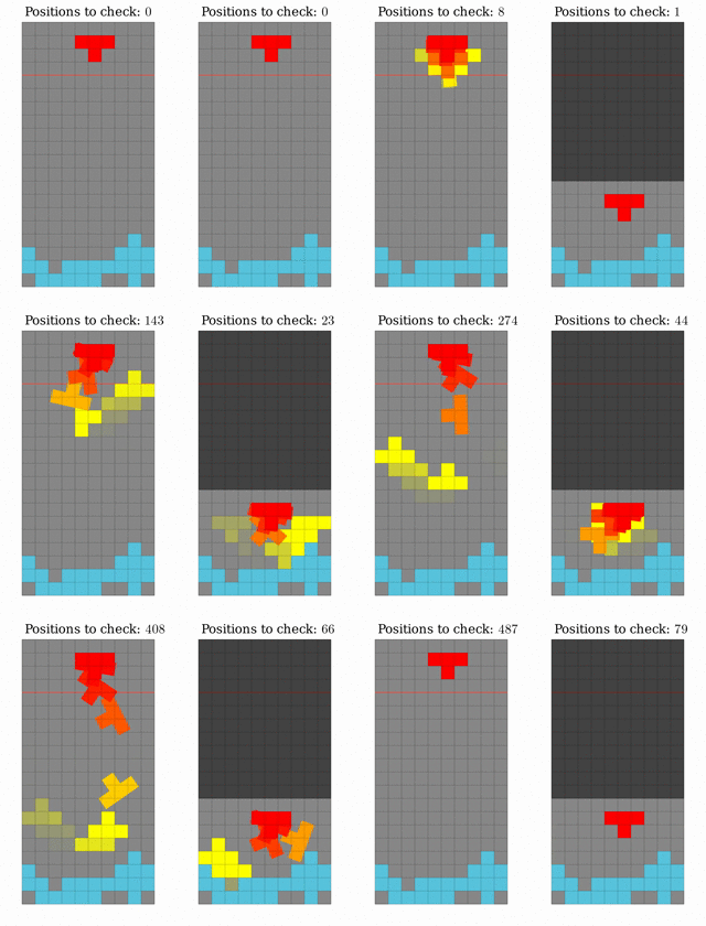 Left: Considering all possible positions. Right: Considering only the positions in the non-empty part of the well.
The next logical improvement was to pre-generate the state graph. That is, instead of starting with the piece in the middle and generating positions for a left arrow, a right arrow, an up and a down, we pre-computed and cached all these states in the “blank” space above occupied rows, which meant we saved significant time trying to compute all these positions, at the expense of having to have a pretty large pre-cached data structure. Fortunately there are only a few thousand starting positions for pieces, which we generated programmatically. It wound up being exactly 2457 positions between all 7 pieces.
In analyzing the performance of move detection, we discovered that the majority of our time was now spent accessing the hash of positions, since whenever a new positions was explored, we had to check if it already existed. A bit of a further dig and we discovered that most of that time was spent running a hashing algorithm on the positions data for comparison. Which again, made sense…but we knew all our positions were unique among each other. We didn’t need to do any hashing, we could just use the position’s representation as a key directly, if we could find a reasonable way to encode it. So we replaced the hashing algorithm with our own custom version that encoded the position as a binary representation of position, rotation and piece type. This was much faster than having to hash a position, and we knew it guaranteed uniqueness. This doubled the speed of our move finder.
At this point, we had a speed of 300 microseconds per core. That’s a ~350% speedup over our initial speed in Rust and a 10,000% speedup over our initial speed in Mathematica. We were confident we’d optimized as much as we possibly could…and still, it wasn’t nearly fast enough. We needed something faster, since all our flamegraphs clearly showed that move calculation was a giant bottleneck in performance. So, we had to pivot.
GPU Matrix Operations
The first idea we came up with was, fitting the theme of this project, a vague notion based on what we had read computers should be able to do. We could just do some matrix math in a GPU!
Our plan was to calculate the legal moves via matrix operations, and speed up those matrix operations dramatically by running them on the GPU. The idea is simple enough: there are a finite number of positions a piece can be in. So, we start with a vector v representing the starting position of a piece, and a matrix M representing all the ways a piece can move from one position to another. The vector v*M (the vector which is the product of multiplying v by M) will then be the vector consisting of all possible positions a piece can be in after one step. v*M² will be the vector consisting of all possible positions a piece can be in after two steps. Do this multiplication n times, and you get v*M^n, a vector consisting of all possible positions a piece can be in after n steps. Eventually, v will stop having new nonzero elements, and then, you’re done - the nonzero elements of v are the positions that the piece can reach in the given well.
vCurrent = startingState
vReachable = vCurrent

while max(vCurrent) > 0:
    vIntermediate = sign(v1.transitionMatrix)
    vCurrent = vIntermediate & ~vReachable
    vReachable |= vIntermediate

return vReachable
There were various improvements and refinements we did with this idea. Instead of using multiplication, we used Boolean logic operators to keep all the numbers either 0 or 1; instead of a full matrix, we had four vectors representing left, right, down, and rotation movements. The math worked, and gave a modest tenfold speedup when tested in Mathematica, but we estimated that in Rust the speedup would be negligible, due to the large number of redundant operations the CPU would have to do. However, GPUs are specifically designed for a large number of simple redundant operations. If we could calculate the legal moves on a GPU, it might provide a substantial speedup.
vCurrent = startingState
vReachable = vCurrent

while max(vCurrent) > 0:
    vIntermediate = permute(vCurrent, leftPermutation)
    vIntermediate |= permute(vCurrent, rightPermutation)
    vIntermediate |= permute(vCurrent, upPermutation)
    vIntermediate |= permute(vCurrent, downPermutation)
    vIntermediate &= vEmpty
    vCurrent = vIntermediate & ~vReachable
    vReachable |= vIntermediate

return vReachable
This required us to get comfortable with difficult topics: writing code to be executed in the GPU via CUDA C and cross-compiling C code so it could run on the GPU. We’ll save the excruciating details of how that worked for the longer post, merely pointing out here that:
- It can be done.
- Make sure you’re writing CUDA C and not C++ or plain C.
- The linker is going to hate you, its not personal, you’ll just have to keep adjusting flags until it works.
In the end, we decided not to go this route, since we came up with another emulator improvement which would provide roughly the same speedup without having to deal with the GPU, which to be honest, had proven quite daunting.
Let Me Count The Waves
Our final approach begun by thinking of the problem differently:
First we considered this: given a specific height, there is a finite set of possible positions that fit within that height. (for example, the height 1-4). These positions are not independent of each other. That is to say, if one piece position is blocked due to a filled square, some other piece positions will be blocked as well. For a given four-line area in the grid, there is a limited subset of potential positions for a piece, considering all rotations and positions within that space. In fact, for every piece except the O piece, there are 34 possible positions (including rotations) in a 4 x 10 area.
A ‘wave’ can be represented as a binary number that is 34 bits, corresponding to the 34 potential positions available to a piece. The binary represents if the position is reachable for the given piece or not. That is to say, if a position is empty and reachable, the corresponding digit in the wave is 1, and if it isn’t, the corresponding digit is 0.
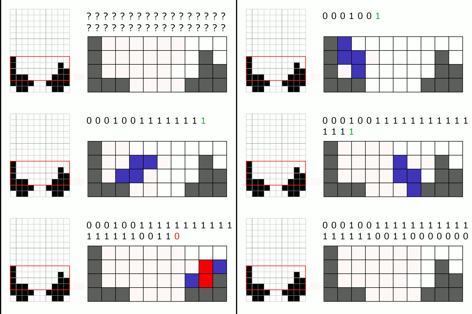
You also have a surface. A surface is the reachable part of a well: That is, any point which has a clear path to the empty top of the well.

The key is that a wave and a four-line slice of a surface, together, form a unique transition: the same wave plus the same slice of a surface will always produce the same new wave one line further down. As a result, the number of possible waves and surfaces is finite, and as we calculate moves, we can store the wave-surface transitions that we encounter in a cache, and the next time we encounter that transition, simply look it up from the cache again, rather than calculating the positions from scratch.
The final result of all this? From an original time of 330 milliseconds per move on Mathematica, to 1.1 milliseconds per move per core in Rust, to an optimized state-based emulator time of 300 microseconds per move per core, we were now down to 48 microseconds per move per core, on average. And, more importantly, finding the positions that a given piece could reach in a given well was no longer the bottleneck; any further optimization would have to be elsewhere.
But why? AlphaHATETRIS was dead, and machine learning wasn’t going to get us there. But the most recent world record holder had some answers for us.
 StickManStickMan #17, by Sam Hughes.
The Era of Knewjade
The Knewjade Heuristic
We’ve talked a lot in the past few minutes about knewjade (Twitter / GitHub). His heuristic. His beam searches. That’s because his work redefined how we were thinking about and approaching the problem. If nothing else, we were sure we could improve upon what he had done. To understand what we did then, it is important to understand what knewjade did to get 66 points, the highest score ever achieved at that point. More than twice what we had once considered an unbeatable 31.
Fortunately, knewjade had published his work, here. While we don’t speak Japanese, Google Translate and staring at pictures helped us understand what was going on.
The knewjade approach is also known as a ‘heuristic beam search’. What does that mean? A ‘beam search’ means that you take some number of positions, get all of their children, keep the best ones, and then repeat the process until you run out of positions. For instance, if you had a beam search with a width of twenty-five million, then at every step, you take the best twenty-five million children from all of your existing wells, and use them as your wells for the next step. The ‘heuristic’ part is how you sort the children from best to worst in order to keep the best twenty-five million of them.
Fundamentally, the knewjade heuristic is a weighted sum of a few different factors. First, holes (empty squares with at least one full square above), and enclosed holes (empty squares with no path reaching to the surface). Holes and enclosed holes are bad. It makes sense that enclosed holes would be problematic: you must clear lines to get to them, and as we know, clearing lines in HATETRIS is no mean feat. Non-enclosed holes are a little more difficult to reason about, but without getting too technical, the layout of a hole can make it impossible or at least extremely challenging to clear, contributing height to the well, without giving an easy means of clearing lines.
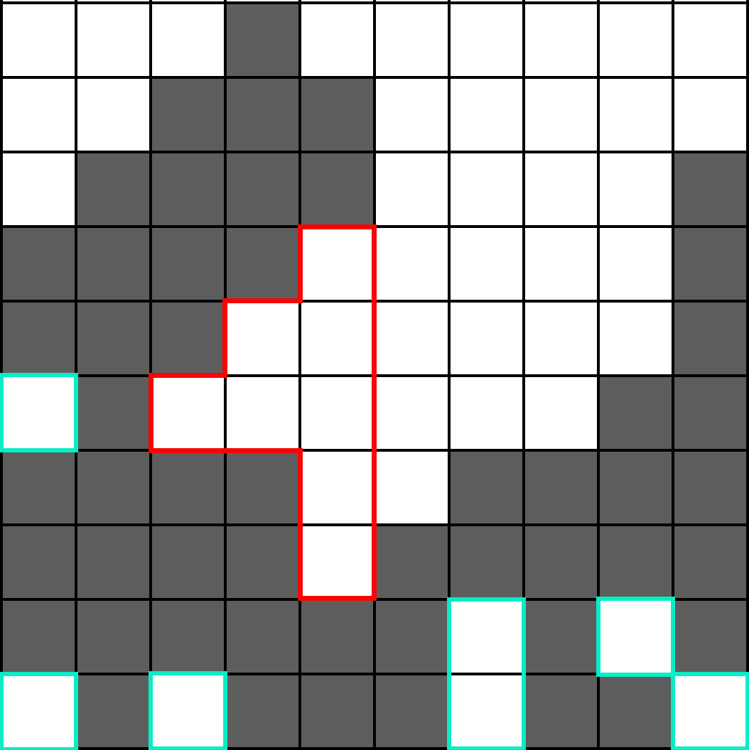 (In red: holes. In teal: enclosed holes.)
Second, the number of lines containing enclosed holes. We’ve already covered that enclosed holes are bad for clearing lines, but not all enclosed holes are created equal. A line with more than one enclosed hole is about as bad as a line with any number of enclosed holes, since you will have to clear all the lines above it regardless of how many holes there are. Thus, we care more about how many lines have enclosed holes, than the number of overall enclosed holes. As an example, the two left wells in the picture below would score quite differently: the one on the top is much more “clearable” than the one on the bottom, since you only have to clear one line in order to be able to access the enclosed holes instead of three.
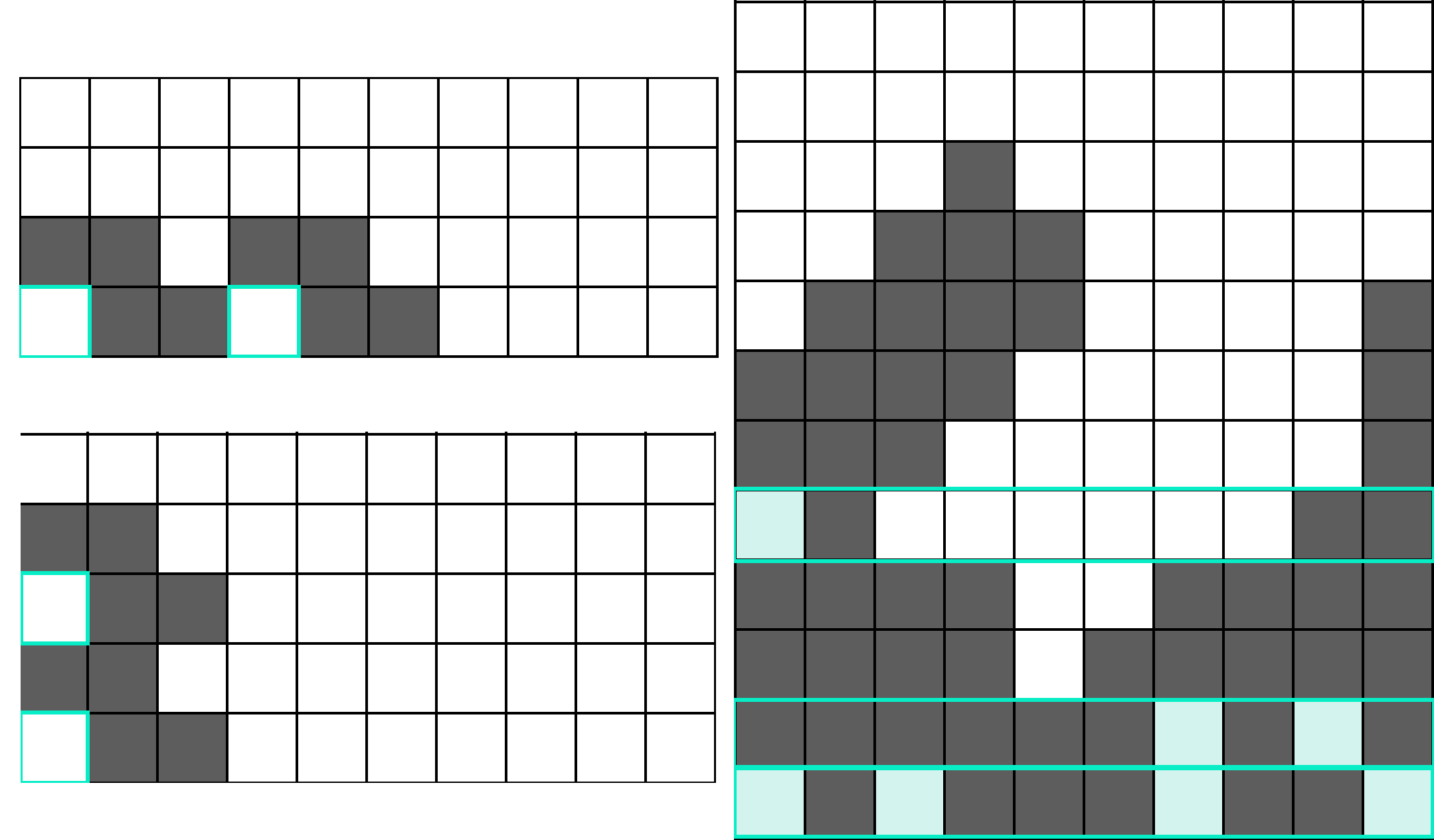 (Left: two wells with two enclosed holes each; the bottom left well is clearly harder to clear than the top left well. Right, lines containing at least one enclosed hole.)
Third, the erasability. How many different pieces can be used to erase a line in this well? The easier it is to erase a line, the easier it is to score. Erasability is good. This well happens to have a very high erasability score, since any piece can clear a line. To demonstrate:
 (A well which can clear all seven pieces)
And fourth, the score. A higher score is good. After all, we want world records. No matter how nice we make a well, all that matters is the score when we inevitably lose.
Each of these factors was given a weight, which knewjade generated with a real-valued genetic algorithm, and the resulting sum was the heuristic: an algorithm to evaluate any well, the higher the heuristic, the better the move.
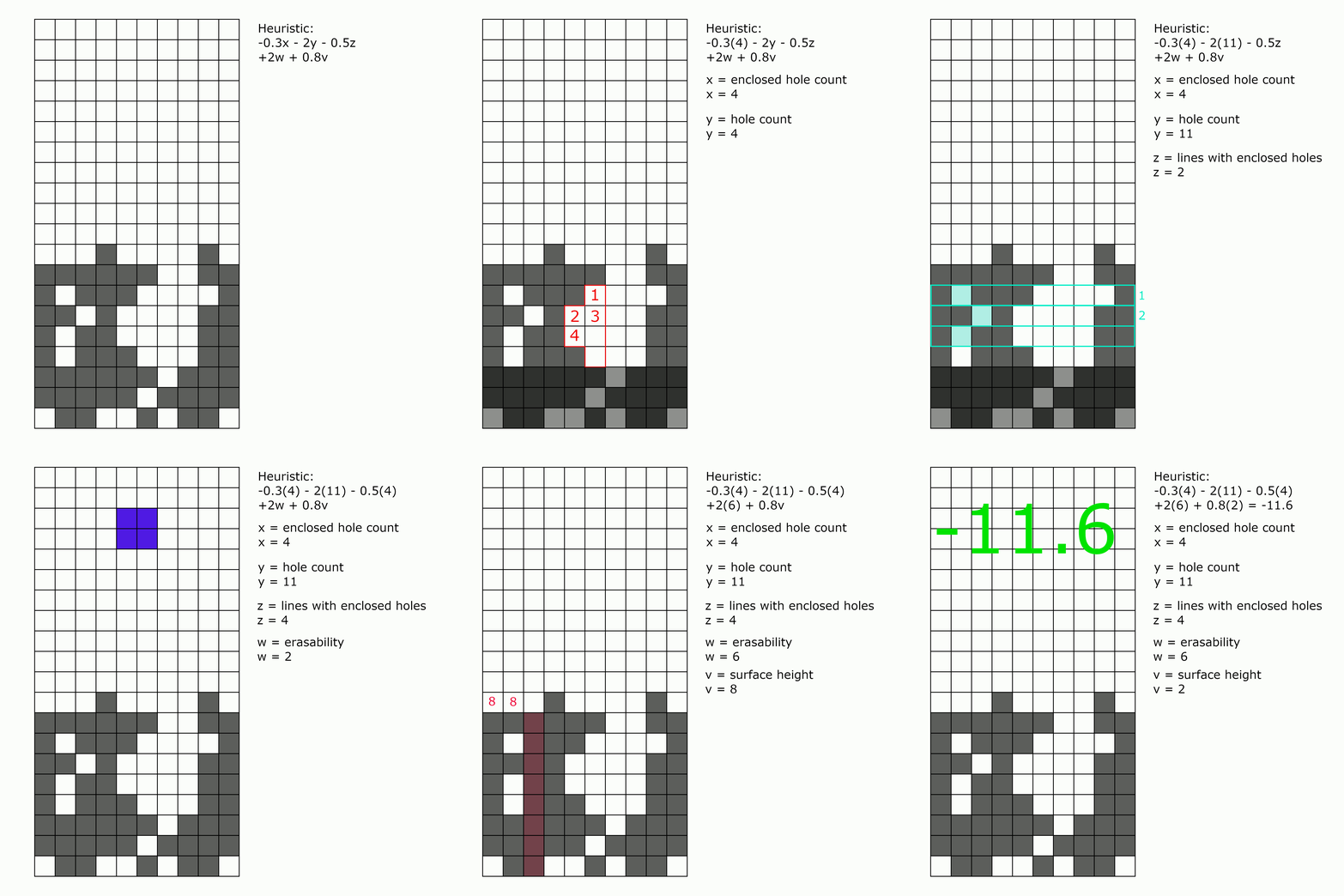
Knewjade had several improvements on this basic concept. One improvement was realizing that, since the surface of a well can almost never move down once it’s moved up, it doesn’t matter how many holes or enclosed holes there are below the surface. All that needs to be considered is the part of the well above the lowest line of the surface. A recap: a surface is the “reachable” part of the well, that is any area that can still be reached from the top.
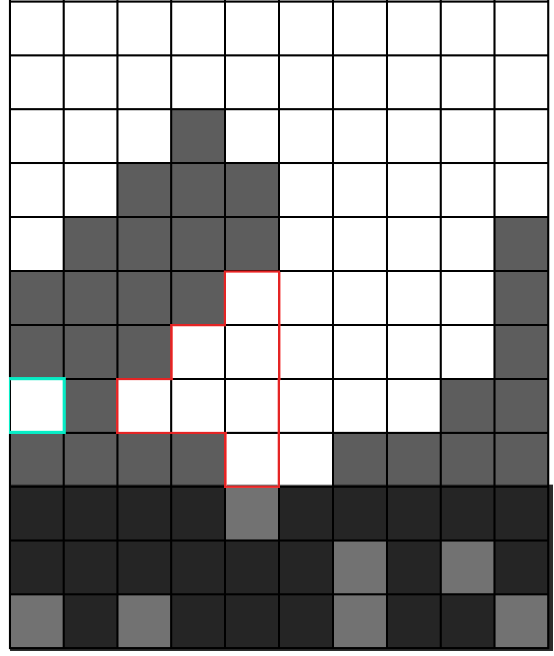
However, there is in general one exception to the ‘surfaces can never move down’ rule: when a line at the bottom of the surface can be cleared with an S or Z piece. So, knewjade’s heuristic doesn’t count holes or enclosed holes if an S or Z piece can free them.
Knewjade’s approach is brilliant, interesting, and innovative, and we were confident we could copy it.
Following Footsteps
So, all we had to do was implement this on our own. And as it turns out, implementing this on our own had a whole host of problems. Our calculation of the surface height took a huge amount of time, and at first, before we discovered waveforms, our emulator was extremely slow, and so calculating the erasability of a given well by calculating all of the legal moves possible for that well was extremely time-consuming. For a while, we thought we could get by without the erasability, and this was a mistake: without the erasability, we could only get a score of 41. Our personal record, for sure, but hardly 66 points.
So, we implemented erasability - but the slowdown was still a huge problem, so we made a second and much larger mistake: we took a shortcut. Rather than computing the erasability for S, Z, O, I, L, J, and T, every single time, we checked if S could be cleared, and only if it could be cleared checked for Z, and then only if Z could be cleared checked for O, and so forth. This sped up the heuristic evaluation significantly (many positions can’t be cleared by all seven pieces), but even when we improved the emulator and no longer had to worry as much about speed, we kept this shortcut in the code. And the problem with that is simple to state: if you’re setting up a well so that you can clear a line, you need to be able to clear that line with all seven pieces, and it does not matter what order you set this up in. We were throwing out perfectly good setups because the setups weren’t in our arbitrary order, and we had completely forgotten that this assumption was bad.
We describe this as a critical mistake, even though it only takes a few sentences to describe, and only one line of code to fix, because it was by far our most time-consuming error, more than any of the tedious debugging for the GPU or multithreading sections. We lost roughly three months due to this, after all was said and done. Knewjade’s beam search had a width of 25 million, and though he could run his in two or three days, we did not have the waveform-based emulator yet, and so our beam search would take three weeks to run. And, with no way of knowing ahead of time how well a given set of heuristic parameters would scale, that’s precisely what we did. Twice. We also had to get the parameters in the first place to test out, which (as we’ll discuss below) also took weeks, and in general we wasted a lot of time looking to improve the wrong parts of the code and not realizing that it was erasability that was limiting us.
Perhaps it’s unfair to blame this one mistake for months of wasted time, because even after we fixed the mistake, our implementation of knewjade’s heuristic was not as good as the original. We know this because knewjade was kind enough to send us his original parameters, and when we ran those parameters - in theory, using exactly the same heuristic he did - the beam search returned a score of 53, instead of the 66 he got. We still don’t know why it was that our heuristic did worse, or what the difference between his implementation and ours was. But by then, we’d come up with an additional term of our own, one which would make replicating the world record of 66 a moot point.
Mumble Mumble Graph Theory
For some months, we’d had a very interesting idea. The idea consisted of the words “graph theory”, which we’d occasionally gravely recite to each other and nod knowingly, with some vague gesticulations, and not much else. Much to our surprise, this turned out to be a workable strategy. Kind of.
While writing and making the visuals for this section, we actually discovered that the graph theory heuristic made no difference at all when used on a sufficiently wide beam search, and that we would have gotten 86 points with or without it. This was in large part because the games we mined for data weren’t representative of the kinds of moves that end up setting world records, and because we didn’t mine enough games to have good sampling rates. However, we include this section anyway, since we suspect that a properly implemented version could be a significant improvement; this heuristic by itself gets 38 points on a 25 million beam search, so setting what would have been the world record before 2021 means that there’s something worthwhile going on.
John Brzutowski, in his 1988 master’s thesis, proved that for a specific sequence of S and Z pieces, it was impossible to win the game of Tetris, and in the process got the ball rolling on making evil versions of Tetris, since it was now a fact that Tetris could, in theory, be so difficult as to be unwinnable. Part of his analysis was looking at the life cycle of “flats” - the creatures occupying individual lines in a Tetris well. These ‘flats’ are composed of blocks and empty spaces, and one could track an individual ‘flat’ from birth when it is nothing more than an empty line in the well) all the way until death (when it is completely filled, and the line goes away).

Brzutowski’s insight was that these ‘flats’ had a very limited number of behaviors each turn. On a given turn, a ‘flat’ can:
- Be born
- Remain exactly the same.
- Fall down a line if there was a cleared line below.
- Grow (gain more full blocks in its line).
- Die (become completely full, and vanish).
So, we can take a full game, and tag each individual flat in the game, watching it as it moves through its life cycle from birth to death - or, move through its life cycle and then stop, permanently. Because, in a game of Tetris that ends, a given flat will at some point either die (get cleared) or reach a point where it never grows, falls down, or changes ever again. The key insight we had was that some line shapes are more likely to die and get cleared than others, and that graph theory could measure and predict this tendency. Essentially there are “good” lines that clear well, and “bad” lines that are really difficult to clear.
In a perfect world where we were furnished with $50,000 a day in AWS credits, we could thoroughly investigate these behaviors over four lines, but with commercial hardware, we could really only focus on one-line transitions. But how do you figure out what makes a line better than its competitors? The answer is where graph theory comes in:

We have in this image a complete set of all transitions for all lines (of width 4; the width 10 transition graph was too big to properly visualize, and even this is pushing it). And, with the data from the tens of thousands of MCTS games we had, it was possible to get a frequency for every transition in this graph, ranging from “vanishingly rare” to “happens almost every game”. There is one starting point – the empty line – and two ending points, not shown in this graph: a flat dying to clear a line, or a flat becoming immortal and never changing again. We could model this.
Model it how? The Ford-Fulkerson method. Imagine the empty well as a source of water, and the two possible end states are buckets. The “water” that travels through the graph all winds up either in a “immortal” bucket or a “cleared” bucket. The frequency of the transitions in the graph, then, represents how ‘wide’ the channel is. Any flat can eventually be cleared, and any flat can become immortal, but if you have a pipe a foot wide towards one bucket and a drinking straw towards the other bucket, the amount of water in each bucket at the end will be different. What we want is to rank how good different flats are based on how much of the ‘water’ flowing through them eventually goes towards the bucket labeled ‘cleared’. This is what Ford-Fulkerson does (in broad strokes, it doesn’t actually model water), and with Mathematica’s implementation of it, we had clearability, the first part of our graph theory heuristic.
The second part was based on similar reasoning. Imagine you have what is frequently an incredible flat when it’s at the top, but the flat is now buried so deep below the surface of the well that no piece will ever reach it. No matter how easy that flat might be to clear in theory, in practice, it’ll never happen. So, we added a second component to the heuristic, permeability. We went through the tens of thousands of MCTS games again and made a second graph, this time detailing which pairs of lines had pieces go from the upper to the lower, and which didn’t.
 (Left: a well which would have a high permeability score. Right: a well which would have a low permeability score.)
So, the graph theory heuristic was the sum of a pair of terms. At each line, the odds that the line would ever eventually be cleared was multiplied by the odds that a piece could get down far enough to get to that line to clear it, with the empty line being by definition the most clearable of all. The higher this heuristic, the better.
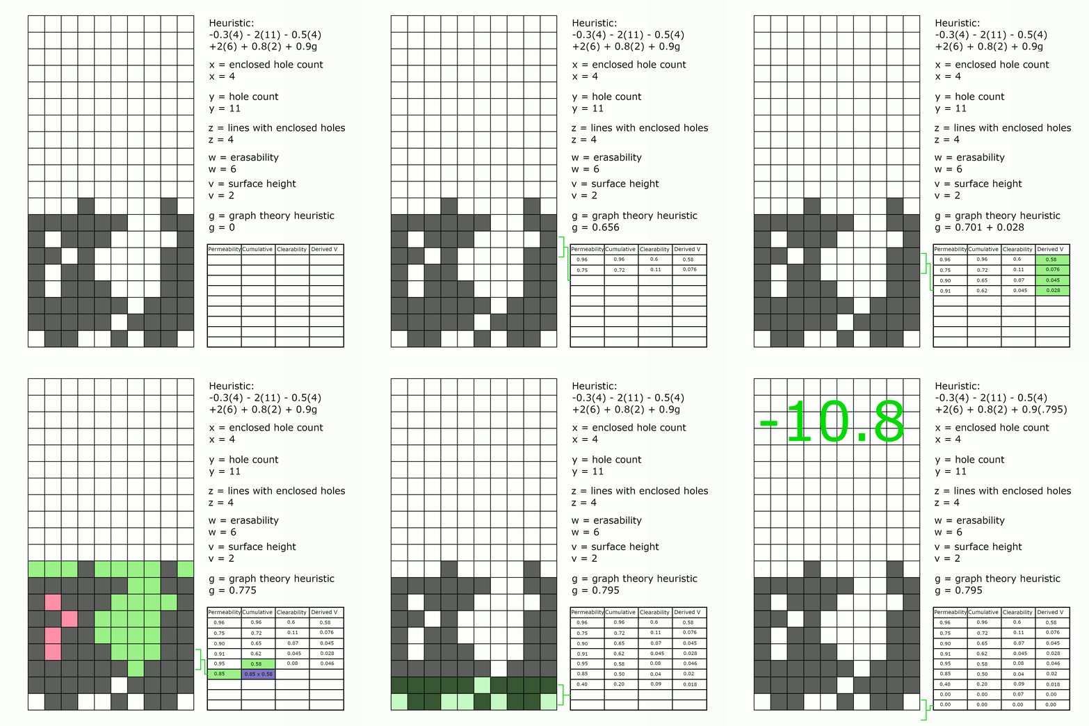
Putting It Together
What we didn’t explicitly say yet, is that these two approaches can be combined. In a very direct way, the knewjade heuristic assesses the quality of a particular well, looking at its shape, considering the piece, and generally calculating its “quality”. The graph theory heuristic, on the other hand, considers only specific lines two at a time, without any broader context of well shape. This joint approach, combining shape and line, gives a more nuanced assessment of the state of the well.
What we suspected (though it’s not something we could formally prove) is that the two pieces should balance each other out. The knewjade heuristic looks at the aggregate shapes in a well – the holes and enclosed holes, the height of the surface – but does so in a general way, with no way of (for instance) determining that this hole is less bad than that one. The graph theory heuristic is quite precise, with thousands of parameters determined from millions of positions, but only considers lines in isolation, or lines in neighboring pairs, with no ability to look at the broader context of the well. Together, ideally, they balance out each other’s weaknesses, and can find better games than either could individually.
(And as mentioned before, on a large enough scale, none of this matters; the additional effect of the graph theory heuristic term drops to zero as the beam search gets wider, and when doing a full 25 million width beam search, it does not matter if the graph theory term is there or not. But that’s not something we’d learn until many months later, and something that might be fixed by improving the data backing our graph theory approach.)
Parameter Optimization
So, with the two parts of the heuristic – knewjade’s, and ours – we were ready to go, and all we needed to know were the weights. By how much should a hole be penalized? By how much should a clearable line be rewarded? How important is score? This last question was especially difficult to answer with just intuition; on one hand, weighting score extremely highly means that the beam search will be very greedy and potentially miss better strategies that take more moves to set up, but not weighting scores highly leads to the algorithm putting off scoring indefinitely, always figuring “Eh, scoring would take away this nice clearable line I found!”. We needed some empirical method to figure out what all these weights should be.
What we found was a Rust library called Simple(x) Global Optimization, a simpler version of the more well known Bayesian Optimization method. This method, like all optimization methods, takes a set of variables (in our case the weights for the heuristic) and a function of that set of variables (in our case, the number of moves a beam search with those weights ran for), and attempts to find the combination of variables that results in the highest value of the function. The upside was that we didn’t have to use any intuition about which weight was more important than which other weight, because Simple(x) could do it all for us. The downside was that this optimization required hundreds of beam searches before we could be reasonably sure we’d tried a broad enough variety.
So, hundreds of beam searches is precisely what we did. With a beam width of 250,000, each search took somewhere between forty-five minutes to two hours, and we let this run for well over a week. Then, after the two failed 25 million width beam searches, and after we discovered the bug, we did the same thing again. By the end, our 250,000 width beam searches had returned a cluster of parameter combinations which lasted for 46 points and 148 moves…and one lone parameter combination which lasted for 46 points and 147 moves, surrounded by very similar combinations of parameters which did much worse.
One of the failed 25 million beam searches had been stuck in a local maximum - the parameters had stumbled upon a game that was good, but that was very difficult to improve upon, like climbing to the top of K2 when you’re trying to climb to the top of Mount Everest. As such, we decided not to go for the cluster that lasted 148 moves, but go for the lone combination that lasted 147, on the hopes of not getting stuck in a local maximum once again.
And we should make explicit here that ‘hopes’ is what we were running on. We simply didn’t and don’t have the hardware to do many ultra-wide beam searches, and the optimum parameters probably change when you enlarge the width by two orders of magnitude. We both doubt very much that this set of parameters is the best possible. All we know is that it scaled up better than any other set of parameters we’d ever used.
| Parameter | Value |
|---|---|
| Holes | 11.2106 |
| Enclosed Holes | 83.7646 |
| Enclosed Hole Lines | 83.7646 |
| Surface Height | -83.7646 |
| Erasability | -83.7646 (per piece) |
| Graph Heuristic | -2.1413 |
| Score | -332.2211 |
(The graph heuristic weight is included for completeness’ sake; do not try that one at home.)
The Final Run
It’s worth talking about what exactly we were using to run these beam searches and machine learning models and various other wild ideas, since to us it felt like every paper we read involved spending tens of thousands of dollars at your local cloud provider. We did not have tens of thousands of dollars to spend. We had about $150 on Azure credits, a machine we’d built a while ago with a slightly modern GPU, an i7 CPU, 16gb of RAM and a motherboard so old it wouldn’t accept any more RAM, and a couple laptops we were using for other things, and occasionally running long simulations on. No more than maybe $2,000 in hardware, being generous and counting the laptops.
Every few weeks as we’d work on the project, we’d read something about how AlphaZero was able to play 44 million games in nine hours and then run them all through neural network training powered by a fleet of thousands of TPUs, sigh wistfully, and look at our machine learning model, which needed another two weeks to finish training on a measly 10k games. Still, by the time we were running 25 million beam searches at the end it wasn’t awful; a beam search would take roughly four days, a vast improvement over the original 6 week runtime (the original beam searches took 3 weeks, but returned games half as long, so would have taken 6 with the better parameters). An agonizing four days, only to get scores like 53, which had once been impressive but were not exactly the world record. Finally, with our best heuristic ready, and all the graph theory mumble mumble was wired up, we decided we’d do it. We’d use a magical cloud machine and be done in a few hours.
We settled on a c5d.18xlarge instance on AWS for $3.50 an hour. The main draw was the 1800 GB SSD and the 72 available cores. With multithreading and some rough back of the napkin math it was slated to take 7 hours. A mere $24.50 for being done. And to be clear, this was our last hurrah. We were considering other ideas, but we knew this was our best shot and that if this failed, we’d likely lack the morale to go back to the drawing board and try again.
Things conspired to delay us. COVID. A stolen credit card. Random real life interrupts. Finally, the Friday of Memorial Day, we spun up the 72 core instance. We’d originally planned on running a few trials on a cheaper 16 core instance… but we opted to skip them. After all, we reasoned, if things would finish in 7 hours, we could reassess after that and see what needed to be changed. We installed Rust, copied files over, set up ssh keys… and then hit run. We’d be well within our budget, $24 being less than the $100 or so we’d budgeted for cloud computing.
An astute reader will probably guess that we did not leave and come back 7 hours later to a world record. Partially because we sat there, glued to the screen, watching games play out, and partially because something had gone terribly wrong. You see, it turns out our back of the napkin math hadn’t accounted for one thing: file reads and writes. Adding more cores made the threaded processes faster, but now the bottleneck was how quickly we could get in and out of the hard drive. And it was not encouragingly fast. 7 hours later we had achieved a score of 10 points at depth 33. Some more quick back of the napkin math suggested we needed probably another 150 moves in order to tie the world record, so another 35ish hours. 42 times $3.50 was only 147 dollars. Still within our mental budget of “no more than $200 of cloud computing”.
Over the next few hours we watched the score inch up, and the depth increase. Never getting as fast as we’d like. It was like watching water slowly, ever so slowly drip into a well, not knowing if it would ever tip over. 10. 25. 35. We still didn’t know if our heuristic could even generate a world record. Watching the score tick up and the cost do the same.
Us being us, we had no patience. Instead of watching it tick agonizingly forward, at around the 48 hour mark, when we were starting to see scores of around 63, we decided we’d cheat - we’d take one well, printed out with the output logs, and run a small 10k beam search on a laptop in order to get a lower bound for how good a game was possible. Like opening presents on Christmas Eve rather than Christmas morning, this did spoil a bit of the dramatic tension - but it also confirmed that we would, at bare minimum, get a score of 71 points, and that we would for a fact get the world record. Somehow this made the remaining ten hours of waiting worse, not better. At the 56 hour mark it finished. We’d done it. We’d discovered a 86 point game was possible, and we were only $196 in the hole. Considering the key-frame generation still had to run to give us the moves that the game had played, we might not even exceed our $250 cloud computing budget.
 StickManStickMan #21, by Sam Hughes.
Key-frame generation? Didn’t we already have a winning game? Well, yes and no. We’d had the moves needed to play the winning game, but we also had billions of other moves that did not lead to the winning game. ‘Key-frame generation’ is how we reverse-engineer a game from a beam search. At each timestep, the beam search saves the top N wells (in this case, 25 million), and stores them all to disk. At the end, we take a well from the last available timestep, go through all of the wells in the previous timestep, and calculate all of their children (though we’ve since figured out a better way). When a well from the previous timestep has, as one of its children, the well we’re looking for, we stop, save that well, and go back another timestep to repeat the process. The process of finding each well reminded us a bit of rendering an animation by generating keyframes, hence the name.
An obvious question here: why didn’t we store the children of each well on disk, so that we wouldn’t have to recalculate the children again? The first answer is that the complete beam search already takes 225 GB of space, and storing the children would far exceed the available space on both the RAM and hard drive. The second answer is that, by the end, the emulator was fast enough that the extra time taken to read the data from disk would have been more than the time taken to recalculate the children.
56 hours in, we had a gorgeous score of 86, assuming there were no bugs in our emulator (an idea which at the time seemed dangerously possible), and all that was left was to wait for the fairly quick process of keyframe generation to finish. It was midnight, and we asked the fateful question “how long can it actually take? An hour?”. This didn’t seem unreasonable, since keyframe generation was usually by far the fastest part of the process. But, as before, we had not considered the issues of scale. The sheer amount of disk reads and the massive depth we’d reached meant that the 72 cores didn’t speed things up at all, since 90% of the time was spent on the single-core operation of reading the timestep files from disk. Some quick math showed that it was going to take us another 12 hours to finish the process. Another 42 dollars and more agonizing waiting. With nothing to be done about it, we went to bed, vowing to wake up in the morning and input the game.
We cannot emphasize enough the sheer frustration at waking up the next day, and seeing it still merrily chugging along, slowly, ever so slowly; the back of the envelope math we’d done had been based on reading files from the end of the search, which were much smaller and faster to read than the files in the bulk of the game. 68 hours in, and the accursed keyframe generator was still only gradually moving forward. Neither of us got to enjoy that Sunday at all, watching it inch forward, bit by bit. Tantalizingly close.
 StickManStickMan #19, by Sam Hughes.
Finally, late that afternoon, it finished. We hopped on a voice call, and put the game in to the online Javascript HATETRIS game, move by move, wondering at each moment if this is where we’d discover a key emulator bug or bad edge case to make all our efforts be for naught. But as the well piled tall on either side, and we fumbled flips here and there, one thing became clear. It was real. The world record was ours. 86 points.
We breathed a sigh of relief. It was done. It was finished. Countless hours of engineering time. Endless runs on our machines, 100 dollars over what we’d originally planned to spend on AWS. (It turned out to be $140 over after data transfer costs and such), but it was done.

Lessons Learned
Up until now, this has been something of a narrative. There’s been a plot, there’s been progress, there’s been a clear (if non-monotonic) improvement from A to B to C. But there’s more stuff we learned, and dead ends we went down, that don’t really fit the story. We’ve captured them here for two reasons. One, we think these are valuable lessons that anyone who dives into this type of problem can benefit from. Two: we did a lot of work, much of which was only tangentially related to getting the world record, and while we’ll save most of that for a future blog post, we want to show some of it off now. These headings will only be loosely coupled, and while we think there’s a few related conclusions, we leave grand sweeping paradigms as an exercise for the reader.
Flamegraphs & Attack of the Clones
One lesson that came up over and over again throughout this project is that profiling is very important, because we as developers are bad at estimating which parts of code are bottlenecks and which aren’t. In one of the earliest iterations of the emulator, we had an error-handling exception which would format and print a string with state information in the event of a panic, to make debugging easier. We quickly fixed the underlying bug which would cause that string to print, but kept the print statement in anyway. What harm could it do?
We had no idea what the relative time cost of any of our code was at that stage, and didn’t find out until later, when we started using flamegraphs (a visual aid showing the proportion of time spent on each function call in a program) to profile our code. We had certain functions we knew for a fact were bottlenecks, so some of the graph wasn’t a surprise. What was a surprise, however, was the mountain sticking up from the surrounding foothills, in the center of the graph:
(Click or hover for more details)
As it turned out, that string format statement was taking up 17% of the total runtime, all in the event of an error that literally never happened. And that was before all of our other optimizations; if we put this string format statement back into the current emulator, it would take up well over 95% of the runtime by itself. And without code profiling, we still would never have guessed this.
Reasoning about runtime is extremely tricky. For all the coding interviews that emphasize calculating the runtime complexity of your program, there is a lot of magic that happens in coding, and the only way to really know what’s going on is to use appropriate tools to detect it. Sure, you should avoid nested for loops inside for loops, but profiling your program can give you even better results.
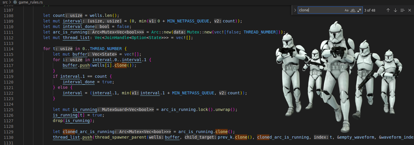
And by the same token, profiling also revealed that we had no need to worry about some things that concerned us. We’d spent significant amounts of time discussing how we were going to fix our various issues with using .clone() to get around borrow issues, and do things properly… but when we looked at the flamegraphs it turns out our 70+ clones were not costing us any time, since they were being optimized away during compilation. What we had assumed was a major time-sink was nothing to worry about at all.
Array vs. BTree
That said, you can’t just ignore runtime complexity, either. Our original version of the beam search took N wells, calculated all of the children of all of the N wells (typically around 15*N), sorted the list, and then took the best N children in the list to use for the next step. This is all well and good for small values of N, but when scaling up, this quickly becomes untenable; storing all of the children at the same time (as opposed to just storing the top N children) wastes a tremendous amount of memory, making the beam search take up on average fifteen times more RAM than it properly should. We knew we had to change something there.
So, we took the obvious route. To summarize in pseudocode:
1
2
3
4
5
6
for well in current_wells:
    for child in children(well):
        if child is better than worst_child in new_wells:
            insert child into new_wells in appropriate_position
            remove worst_child from new_wells
            get new worst_child from new_wells
And therein lay the problem, though we didn’t figure it out for another month and a half. Reading an arbitrary element from the vector is O(1), but insertion into the middle of a dynamically-sized vector is not an O(1) operation - it’s O(n), scaling with the number of elements in the vector. This caused a huge nonlinear increase in runtime with respect to the beam width; had we tried to do a full 25 million width beam search at this point (and we wouldn’t have tried), it would have taken literal years to finish even with Rust’s impressive compiler magic.
We briefly considered using linked lists, despite well-known warnings about how tedious and difficult they could get in Rust, but linked lists presented a different problem. Insertion in between two elements is nice and fast at O(1), but reading through the linked list to find out where to insert is O(n). This was exactly the opposite of the situation with vectors, but it was no closer to being a solution.
Upon seeing that we had two data structures, one which could read quickly but insert slowly, and the other which could read slowly but insert quickly, we thought “surely there’s some sort of compromise data structure that does both pretty well”. And sure enough, there was. Rust’s BTreeSet was a built-in data structure based on B-trees, which have logarithmic read times and logarithmic write times. Things were slow enough already that we were willing to accept almost any constant in front of those logarithms, so we switched, and went from insertion taking up more than 90% of the beam search runtime to less than 1% instantly.
| Data Type | Insertion Time | Element Read Time |
|---|---|---|
| Vector | O(n) | O(1) |
| Linked List | O(1) | O(n) |
| B-Tree | O(log(n)) | O(log(n)) |
Changing the datastructure was the key to unlocking larger beam searches, but this would have been futile without the improvements we got from the flamegraphs, and in turn wouldn’t have worked if we’d spent all our time cleaning up clones. Writing highly efficient code is more of an artform than a science (and we await a flurry of angry tweet from our many reader over this statement). It requires a mix of the right tooling, understanding your code, and figuring out what tradeoffs make sense.
Machine Learning (on the cheap)
There’s another lesson we learned as we optimized our code as best we could…no amount of optimal code will eliminate the need for absurd amounts of hardware for machine learning. It doesn’t matter how good your emulator is, how blazingly fast you can play games… the sheer amount of training data and training time needed makes trying to solve problems of more than trivial complexity on consumer hardware very very challenging.
We’re not machine learning engineers. We don’t have formal backgrounds in machine learning, or in anything remotely close. Mr. Hughes generously said that we “appear to be academic researchers”, but that appearance is purely surface level. It’s possible, as it always is, that we were just doing everything wrong, and someone with a PhD in applied machine learning will show up with a model far better than any beam search we’ve designed. We wish for nothing more. We want user friendly machine learning for amateurs like ourselves. In fact, when we set out on this project, one of the things we wanted to prove was that AlphaZero could be used for a practical purpose without a massive computing cluster. As far as we can tell, it cannot.
The cloud costs, in TPUs and GPUs and RAM, to really get this project off the ground would have been considerable. Our models, tiny and poor as they were, still took two plus weeks to train on a very low number of games, and one of the things we’ve realized is that machine learning depends on having vast reams of data. It’s not sufficient to have 100,000 good games; you need tens of millions. And you need to be able to take games generated by your models and train on them. With super slow hardware, its impossible to tweak hyperparameters to figure out the best learning approach. (Which is, as far as we can tell, how the big, successful projects figure out their hyperparameters, careful guessing, and a lot of tweaking.)
Its frustrating to learn that the incredible tools that are supposed to revolutionize problem solving are out of the reach of anyone not able to throw significant cash at it. There’s a whole possible blog post on this topic. We’re hardly the first to realize it, but we felt it extremely keenly.
Behaviors at Different Well Heights
Since we had an emulator handy, while we were waiting to get sufficiently good heuristic parameters for the full case, we thought to explore some smaller wells, and see if there was any obvious trend in maximum score and maximum game length we could extrapolate. The primary motivation behind this was simple: before embarking on programs which would take weeks or even months to run, we wanted to prove to ourselves that knewjade’s record of 66 was beatable, and that it wasn’t simply the maximum possible score attainable in HATETRIS. So, we did a series of breadth-first search runs, up until it exceeded the RAM available on a laptop, and wrote down the results.
10 Blocks Across
| Height | Score | Length | BFS Width |
|---|---|---|---|
| 0 | 0 | 0 | 0 |
| 1 | 0 | 0 | 0 |
| 2 | 0 | 4 | 21 |
| 3 | 0 | 6 | 310 |
| 4 | 1 | 11 | 9095 |
| 5 | 4 | 19 | 174634 |
| 6 | 8 | 31 | 4848325 |
| 7 | 12 | 43 | 141514270 |
| 8 | ≥17 | ≥57 | ≥1.00e8 |
| … | … | … | … |
| 16 | ≥86 | ≥247 | ≥2.50e7 |
This set of runs had some interesting results. Among other things, we had assumed (and we were not the only ones) that since there were 10*16 squares in the grid, each one of which could be either filled or not filled, that there were roughly 2^(10*16) ≈ 10^48 possible HATETRIS wells. However, here, the results indicated that the number of possible wells was vastly less; the maximum width of the BFS search increased by a factor of ~30 with each additional line of height, so the maximum number of concurrent states would be somewhere around 10^20:

For a game lasting (say) a thousand moves, this would be at most 10^23 possible wells. This was twenty-five orders of magnitude less than we expected, though sadly it was still nine orders of magnitude or so beyond what we could do with commercial brute-force and commercial hardware.
For completeness’ sake, we also examined narrower wells, to get as much of a feel for the behavior of HATETRIS with respect to well dimensions as possible. Width 4 is a special case, since an infinite loop there is actually possible in our emulator (and not possible in the newest version of HATETRIS); there’d be no point going any further. Doing BFS for wider wells might be interesting too, but our emulator currently can’t go beyond 10 blocks across, so we left that as a problem for a future date.
EDIT (May 22nd, 2024): The original values here were incorrect; this version of the emulator had a bug that only occurred when the well height was reduced; in certain circumstances, a piece which filled a line while sticking out the top of said line would be counted as a clear, rather than ending the game. That has been fixed, and these should hopefully be the correct values.
8 Blocks Across
| Height | Score | Length | BFS Width |
|---|---|---|---|
| 0 | 0 | 0 | 0 |
| 1 | 0 | 0 | 0 |
| 2 | 0 | 3 | 10 |
| 3 | 1 | 6 | 75 |
| 4 | 1 | 8 | 1172 |
| 5 | 5 | 17 | 12447 |
| 6 | 6 | 21 | 159942 |
| 7 | 9 | 28 | 2250610 |
| 8 | 11 | 34 | 31440780 |
6 Blocks Across
| Height | Score | Length | BFS Width |
|---|---|---|---|
| 0 | 0 | 0 | 0 |
| 1 | 0 | 0 | 0 |
| 2 | 0 | 2 | 4 |
| 3 | 0 | 3 | 21 |
| 4 | 1 | 6 | 142 |
| 5 | 2 | 8 | 682 |
| 6 | 5 | 13 | 3998 |
| 7 | 6 | 15 | 23337 |
| 8 | 8 | 19 | 149389 |
| 9 | 9 | 23 | 1017165 |
| 10 | 12 | 28 | 6995425 |
| 11 | 13 | 32 | 50825005 |
4 Blocks Across
| Height | Score | Length | BFS Width |
|---|---|---|---|
| 0 | 0 | 0 | 0 |
| 1 | 0 | 0 | 0 |
| 2 | 0 | 1 | 2 |
| 3 | 0 | 2 | 5 |
| 4 | ∞ | ∞ | 16 |
5 Blocks Across
| Height | Score | Length | BFS Width |
|---|---|---|---|
| 0 | 0 | 0 | 0 |
| 1 | 0 | 0 | 0 |
| 2 | 0 | 1 | 3 |
| 3 | 0 | 2 | 8 |
| 4 | 1 | 4 | 41 |
| 5 | 3 | 7 | 134 |
| 6 | 4 | 10 | 543 |
| 7 | 5 | 12 | 2150 |
| 8 | 6 | 14 | 8670 |
| 9 | 7 | 16 | 35017 |
| 10 | 8 | 19 | 148656 |
| 11 | 10 | 22 | 645397 |
| 12 | 11 | 24 | 2935961 |
| 13 | 12 | 26 | 13436407 |
| 14 | 13 | 29 | 61699120 |
| 15 | 15 | 32 | 285071640 |
6 Blocks Across
| Height | Score | Length | BFS Width |
|---|---|---|---|
| 0 | 0 | 0 | 0 |
| 1 | 0 | 0 | 0 |
| 2 | 0 | 2 | 4 |
| 3 | 0 | 3 | 21 |
| 4 | 1 | 6 | 139 |
| 5 | 2 | 8 | 679 |
| 6 | 4 | 12 | 3973 |
| 7 | 6 | 15 | 23126 |
| 8 | 7 | 19 | 143175 |
| 9 | 8 | 22 | 979997 |
| 10 | 11 | 27 | 6771901 |
| 11 | 12 | 30 | 48488721 |
| 12 | 15 | 36 | 362642476 |
7 Blocks Across
Finding The Bug
Along the way, trying to come up with optimizations for this state-based emulator, we encountered an interesting bug. ‘Interesting’ because the original implementation of HATETRIS briefly had exactly the same bug, and had it for exactly the same reason:
Start a new game and hit “rotate” four times. Note what happens to the piece. Unlike many Tetris games, the rotation process is actually mathematical; each new piece rotates around a “point of origin” which is at the junction point of four squares. The rotation is performed by fiddling with the actual coordinates of each of the four “bits” which make up the piece. Each piece actually has a point of rotation in addition to everything else.
The algorithm which tests all the possible positions, actions and final resting places of each possible new piece can do anything you can do: left, right, drop, rotate. The algorithm stores a list of all of these locations and applies all possible transforms to each location in turn in order to generate a complete list. Obviously, each new location thus generated has to be compared with the whole list to make sure it is new. One of my early attempts to make the algorithm faster made it so that it only checked the locations of the four bits, not the central point of rotation.
However, in the case of an
SorZpiece, the point of rotation is significant. Hitting “rotate” will result in a different piece depending on which way up the piece is. In Tom’s 12-point run, the algorithm moved anSpiece to the same location as he did, and hit “rotate”, but because the piece was the other way up, resistance was encountered and nothing happened. With the piece the other way up, which is what Tom did, the rotation is successful and a line is made.
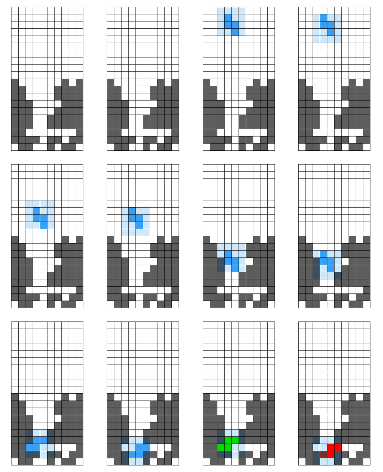
In other words, an S or Z piece occupying the same space can in fact be different pieces with different available positions. This means that the optimization of only considering the space a piece is taking up, rather than storing properties like ‘rotation’ and ‘position’ separately, will end up failing in some edge cases. This wouldn’t have been a huge speedup, and it’s not that important, but it was a signal to us that we were slowly but surely following the same path.
Echoes of AlphaZero
The core premise of the AlphaZero neural architecture is that it is dual-head: the neural network has a policy head, and a value head, and the formula for determining which moves to investigate uses both. The value head is the simpler of the two: it takes in a position and outputs a single number ranging from -1 (meaning a predicted 100% chance of defeat) and +1 (meaning a predicted 100% chance of victory). The value head is what allows the algorithm to decide how good a position is, without having to play the entire game through to the end.
 StickManStickMan #691, by Sam Hughes.
The policy head can be thought of (in very broad strokes, don’t take this too literally) as the ‘gut feeling’. If you’re a chess grandmaster, you don’t play as well as you do by looking at every possible move and counter-move that could be made - the branching factor of chess is simply too high. Instead, your gut feeling tells you to look at moves X, Y, and Z, so you do, and you don’t consider (or only briefly consider) the dozens of other possible moves available. The policy head works something like that, biasing the algorithm so that it does not consider all moves and all branches equally.
What we did, combining the overall ‘board sense’ from the knewjade heuristic and the line-by-line precision from the graph theory heuristic is very, very far removed from the original AlphaZero algorithm. Nevertheless, we couldn’t help but be reminded of the balance that the policy head and the value head were supposed to bring to each other when combined.
(This section was written long before we discovered that the graph theory heuristic made no difference; our intuition is no more perfect than the policy head’s.)
Reversing the Polarity
Keyframe generation took quite a while on the world record run, due to the sheer amount of time needed to read hundreds of gigabytes from disk into memory. There’s a better way to do it that didn’t occur to us until afterwards: make the emulator run backwards. That way, rather than calculating every child of every well that’s saved, simply calculate all of the possible parents of the well directly, and see which of those parents is in the previous generation’s well list.
If we really needed to speed up the process even further, we would write to a disk database rather than writing each timestep as its own file, and then when calculating the keyframes we’d only have to search the disk database for the dozen or so possible parents of the current well, probably getting the complete game in a few seconds.
Unfortunately, the initial idea of taking this idea to the extreme and calculating the entire ‘reverse game tree’ didn’t work; looking further than ten or so moves is currently very impractical, since most possible parents of a well are not reachable HATETRIS states (going back to the earlier discovery about how few reachable HATETRIS states there actually are). It’s possible to filter out some of the unreachable states (for instance, any well that has a partially filled line above a completely empty line is definitely unreachable), but we couldn’t figure out a way to filter out all of the unreachable parents, or even most of them, and so the effective branching factor is too high. If a full reverse emulator is possible, it would potentially allow for diskless beam searches, but right now it’s a bridge too far.
The Next World Record
We never bothered writing a script to take a list of wells and turn it directly into a valid Base2048 replay; it wouldn’t have been that difficult, but it was never important enough to actually get done. Instead, we printed out the list of wells, went through them one by one, and manually hit the arrow keys on the Javascript version of the game to move each piece where it needed to go. And along the way, we noticed a trend, one that we noticed also in knewjade’s 66 point run.

The winning game piled pieces up pretty high, and did so pretty early; it first had a piece touch the top of the well less than halfway through the game (move 120, for a game that lasted 247 moves). Looking at it, it makes sense that piling up pieces benefits the score; the HATETRIS algorithm is based on the height of the well, so maximizing the well height minimizes the amount of information the HATETRIS algorithm has at its disposal, and puts an upper bound on how evil its piece selection can be.
So by that logic, a perfect game should keep pieces piled all the way up to the top the whole time. Ours does not - our heuristic indirectly penalizes wells for being too high, because stacking pieces all the way up to the top takes time which could be used to score points and clear lines. And any well which goes too long without clearing any lines tends to get filtered out. The left-hand side of that graph is a land of opportunity, and a better heuristic than ours could probably get more than a hundred points by properly exploiting it.
Going back to the analysis on smaller wells, the length of the best possible games seems to increase approximately quadratically. Fitting a quadratic function to the results from well heights 2 through 7 and extrapolating out (and taking the result with a grain of salt), we’d expect the best possible game to last about 290 moves, which, like the previous estimate, would correspond to a best possible score of 102-103 - at the very least, indicating again that the current record is not the best possible game.
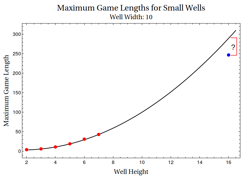
86 points is not the end of this story. It is, however, the end of this blog post.
Specific Thanks
- Arta Seify, for writing his thesis on modifying AlphaZero for single-player games, and for helping us quite a bit with implementation details when we emailed him.
- Dr. Antoine Amarilli for inspiring the small well size experiments.
- Kevin P. Galligan, for providing insight into what alternate routes there were besides beam searches and MCTS to making a HATETRIS solver, and how far those alternate routes can get.
- David’s dad, for suggesting B-Trees rather than linked lists or dynamic-sized arrays.
- えぬ・わん, for making a video analyzing the strategy used in our world record; more analysis than we did ourselves.
- Aypical, SDA Guest, Ivernis, Deasuke, and chromeyhex, for giving HATETRIS a proper leaderboard and for each setting the bar successively higher.
- Knewjade, for setting forth both a monumental challenge and the tools needed to eventually overcome it.
- Sam Hughes, for getting us to waste fourteen months and fourteen thousand words on Tetris. So far.
P.S.
Ok, so we lied about that last part being the end. If you read this far, (which is, lets face it, unlikely) you’ve heard a lot of griping, seen some things that look semi-magical, and possibly left with the impression that the authors had some sort of incredible knowledge base, or are researchers deeply entwined with the topic.
We’re not. We’re not researchers at all. We’re just two people who became obsessed with a problem and put their meager knowledge to use, beating rocks against rocks in different configurations until something resembling a spearhead came out. Our experience with Rust was, up to this point, six blog posts done on introductory Advent of Code problems over the course of six months. We didn’t know much at the start, but we learned. First, we Googled and clicked on the first result. Then we scoured Stack Overflow and papers, and when that failed, we reached out to specialist Discord servers and emailed experts. When existing Rust crates didn’t do what we needed, we made our own Rust crates. We now know a lot of very obscure information about HATETRIS, but you could still fill volumes with things about HATETRIS that we don’t know. Many of the breakthroughs we had were due to ignorance. We pulled out the concept of waveforms because we were terrified that the next thing we’d have to do to push things forward was do complex matrix operations on a GPU. Inventing a new way of thinking about the problem seemed easier.
You, too, can do something like this. Find a problem. Become obsessed with it. Learn everything you can about it. Fall down dead ends. Give up, and then keep thinking about the problem at night. Have Eureka moments that lead you down other dead ends. Find a friend willing to get as obsessed as you are. Underestimate the time commitment, and then refuse to back down. Embrace the sunk cost fallacy. As long as you keep thinking about the problem, even if its in short bursts every few years, you’re still making progress. And if you never finish? If all you find are side-paths and obstacles, and it turns out the entire mission was doomed from the outset? That’s okay too. Projects like this nourish us, because there’s a part of the human mind that wants nothing more than to climb the mountain, rappel into the cave, explore the unknown and grapple with it.
So, regardless if you’re here because you care about the technical details, or because you saw HATETRIS and said “I heard of that, I think”, if you only take one lesson away from this whole thing, we hope it’s this. You too can do the thing you think is impossible or difficult.
If you fail? Write about it anyway. The original title of this post was “How Not to Get the World Record in HATETRIS”.
 StickManStickMan #620, by Sam Hughes.
Comments powered by giscus.
