Trackmania III - The Eyes

Series Navigation

Trackmania is a video game, and though it can be played without a monitor, or blindfolded, it was designed with the assumption that the players could see what they’re doing. So our first step, now that the nightmares of setup were over and the actual work could begin, was to give our nascent network a way to see the game. The goal throughout this project has been to make a bot that learns as fast as a human does, so we wanted the program to learn from the kind of graphics that human players use, eventually deciding to give our bot an image input with a resolution of 1600x900, at 30 frames per second.

In the end, we proved that this goal is possible, but a full implementation was beyond us.

Image Acquisition

We need to use each frame for two purposes: driving and training.

Driving: It is obviously important for the program to know where it is going, so the program needs to decide which way to steer the car, every 33,000 μs. Thus, we need to get the image to the neural network for processing in much less than 33,000 μs, because the program will need time to process the image, make a decision about which keys to press, and send the keypress decision to Trackmania.

Training: The program needs to learn from prior runs, minutes or hours or days from now. If we want to ever generalize and have a program that can learn new maps, the network will need periodic reminders of previous maps, or else risk overfitting to whatever map it happens to be playing right this second. You can think of this as the memory of past races.

So, we need an image, and we need the image in two places. We need it wherever the neural network is, and we need it wherever a large amount of data can be stored for a long time.

Screenshots from Disk

The easiest framegrab method to implement is also the most obvious one. Trackmania 2020 has a built-in screenshot function accessible with a single keypress (F12), which saves a picture of the game to a specific folder on the hard drive. Failing that, most operating systems have functions (usually mapped to Prt Sc) which take a picture of the entire screen and save it the same way. So, the easiest way to get the pictures of Trackmania is to press a screenshot button continuously (using whatever technique you’re using to send keypresses to steer the car), and have your program scan the folder and load any pictures that weren’t there 1/30th of a second ago into the RAM, where your program can use it.

This isn’t as silly an idea as it might seem. If we’re going to be storing large amounts of data for future training, the hard drive is the natural place to store it. And if we’re going to be storing data there eventually, why not put the screenshot there to start with?

The primary problem with this approach is that data transfer to and from a hard drive takes a long time. We have 33,000 microseconds for the entire frame-by-frame decision-making process. Preliminary timings for our 1600x900 screen showed that it took on average 16,000 μs to save a screenshot to disk and 21,000 μs to load the screenshot from disk again, for a total of 37,000 microseconds - 112% of our time already gone.

And even that’s a generous estimate; that assumes that the screenshot is taken at the exact moment of a frame update, which we are not (yet) doing anything to ensure. If the screenshots and the game are out of sync with each other, then there could be another delay between 0 and 33,000 μs added on top of that, for an average 52,000 microsecond total delay between when the frame is rendered and when the neural network can even start to process the screen for its own decision-making; by the time the network even begins working a frame, the game will have already displayed the next one, and be on the verge of displaying the one after that.

This wouldn’t be a dealbreaker for 10 FPS or 20 FPS, but for 30 FPS, it’s too much of a delay. Linesight got around this problem by taking tiny screenshots and keeping them all in RAM, but our screenshots are 225 times larger than the 160x120 greyscale images; if we tried to do the same thing and keep full-resolution images in RAM, we would fill up 64 GB of RAM in less than ten minutes.

Obviously, we were going to have to come up with something else.

Screengrabs from RAM

If we need the screenshot from disk, but we first needed to save it to disk, it makes sense to ask if we could cut out the middleman. Rust does have crates for this, and the crate we decided to test was nvfbc; it has the option of viewing the contents of the screen directly from the frame as stored in RAM, with no need for any hard drive reading or writing. The average timing - correct this time - was 1,300 μs.

This is one example that shows why we picked Rust and Linux over the (theoretically easier to work with) Python and Windows. This is a racing game. We wanted to write a program that is fast. When the Linesight project faced the same problem we did and needed to get images from the screen to the neural network quickly, Agade09 found that none of the existing screenshot-to-memory tools in Windows were fast enough to suit the project’s needs, and wrote his own custom library, DXCam, more than twice as fast as any other Windows / Python screenshot tool.

For a full-sized 1440p resolution, DXCam provided a framegrab rate of 238 FPS, for an average screenshot time of 4,200 μs. A standard 1440p resolution has 2.56x more pixels than a 1600x900 display, so as a first-order approximation we’d expect that to translate to 1,600 μs for our display. We got 1,300 μs right out of the box, without having to write our own library.

We wrote our own library anyway. But we’ll get to that.

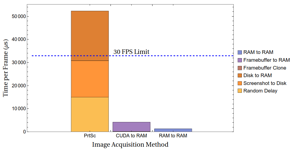
Image Processing

Linear Layers

The most basic type of layer for a neural network is a fully-connected linear layer, in which all of the inputs are fully connected to and contribute to all of the outputs. Each contribution from an input to an output consists of a multiplication and two additions, for a total of four floating-point operations each. Our input consists of 1.4 million pixels, each containing three values (red, green, and blue), and our output consists of some number of neurons in a hidden layer. That’s 24 million floating-point operations per hidden neuron. How long would that take?

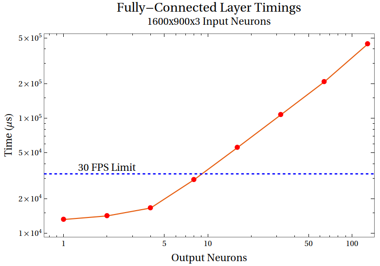
It takes somewhat less time than we expected when we wrote this benchmark. CPU caching evidently speeds up the process tremendously, even without tricks like SIMD that could be used. However, it’s not fast enough. The landmark 2012 paper ImageNet Classification with Deep Convolutional Neural Networks has a hidden layer consisting of 4096 neurons. From our timings, we could have a hidden layer consisting of at most…ten neurons. The maximum amount of information about the picture given to the rest of the network is bottlenecked by the number of hidden neurons, and so we certainly need more than ten numbers to describe the screen in enough detail to make good decisions.

Somehow, we need to reduce the number of operations needed to process an image. Fortunately, that same paper shows how to do it.

Convolutional Layers

Intuitively, a fully connected linear layer with all pixels contributing directly to all hidden nodes feels like overkill.

Take an image, and shift it one pixel to the right. That image hasn’t changed much. Most of the features that were there before are still there now. But, to a fully connected layer, this new image is completely different than its predecessor image, shifted one pixel over. If the network has learned about the importance of a red pixel at position (474, 1337), it will have no idea that a red pixel at position (474, 1338) is in any way similar to it. The network would learn the significance eventually, given enough data and enough processing power, but it doesn’t seem as efficient as it could be.

The basic intuition behind a convolutional layer is that there are many features of an image that are local and translation invariant, meaning that the features are small (relative to the size of the entire image) and are the same regardless of where in the image they are. The excellent machine learning textbook Dive Into Deep Learning uses the analogy of a Where’s Waldo picture: Waldo is small, and what Waldo looks like is not dependent on where he is. A fully connected layer would not be the best way to find Waldo in a huge picture; a better way would be to have a ‘Waldo detector’ (which determines if Waldo is or is not in a small picture), break the large picture up into many small pictures, and then run the ‘Waldo detector’ on each one of the small pictures.

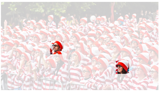
That is, in essence, what a convolutional layer does. A convolutional layer consists of a number of convolutional filters, each of which detects some small feature of the image wherever that feature happens to be. One filter might detect right-edges, and another might detect left-edges, and a third might detect a fuzzy pattern that makes no sense to us as humans. When you stack these features together, you’re able to identify a specific image or feature in an image that is essentially the sum of these things.

A normal image has three channels: one for the intensity of red pixels, one for the intensity of green pixels, and one for the intensity of blue pixels. A convolutional layer will take these three input channels and produce some number of output channels. So, to identify Waldo, you might look for high intensities in the red fuzz channel, white horizontal line channel, blob shape channel, smile shape channel, and flesh color channel, all in the same place.

And that’s the real strength of the convolutional filters: you can do this over and over. Take all those channels (red fuzz, white horizontal line, and so forth) that were output by the first convolutional layer, and input them into a second layer. One of the channels output by that second layer might be a ‘Waldo-ness’ channel, and the intensity of the pixel corresponds to how likely that pixel is to be part of Waldo. Another channel’s intensity might represent the ‘car-ness’ of a given pixel, and another’s might represent the ‘tree-ness’. Stack these convolutional layers on top of each other, and you can detect higher- and higher-level features of the original image. That’s the goal. We want a neural network that can recognize obstacles, and distinguish between surface types, and aim towards finish lines. One layer isn’t enough.

So, how many layers do we need? We have no idea. We’re going to see how many we can handle, and go from there.

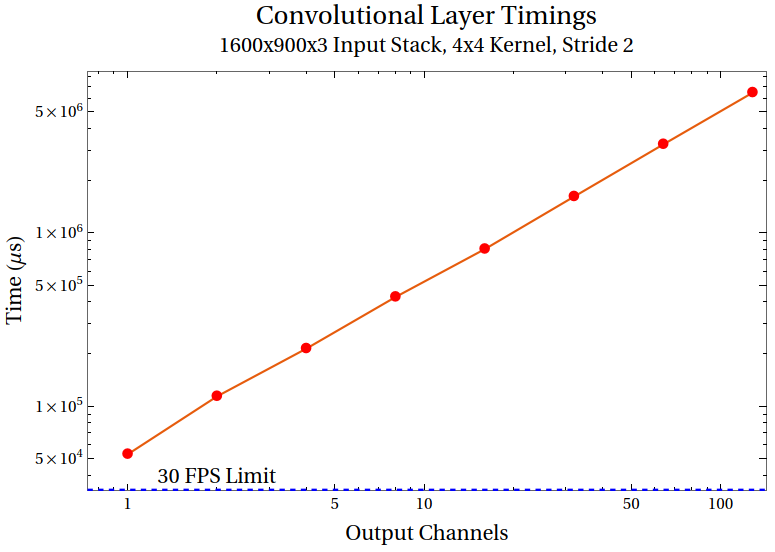
What we found: it takes much too long, even in the smallest possible case, to compute even a single convolutional layer. Note the difference in x-axis between this graph and the previous one: we’re now measuring not output neurons, but output channels; for a stride of 2 and an input size of 1600x900, that’s 800x450 output neurons per channel. Compared to a linear layer, there are far fewer calculations per output neurons…but far more output neurons. We can’t even come close to a single output channel for a full-resolution image, if all we have is our CPU implementation of convolutional layers.

But, the convolutional layer involves doing the same handful of operations, in parallel, over and over again. GPUs are specifically designed to do the same handful of operations, in parallel, over and over again. The natural question to ask, then, is: can this be done on the GPU? And if so, how much of an improvement would it be?

cuDNN

Our GPU is an NVIDIA RTX 2070; since it’s NVIDIA, the most natural programming language to use to run tensor operations on our GPU is CUDA. One of CUDA’s libraries is cuDNN, which provides functions for running deep neural networks on a GPU. And, luckily for us, someone already made a Rust crate giving access to cuDNN. All we had to do is figure out how to use it, and how to send tensors to and from the GPU in a format that cuDNN could read.

Even more luckily for us, the same nvfbc crate we used to capture the screen contents from RAM could also capture the screen contents from the internal GPU buffer. The GPU framebuffer itself is protected, and can’t be modified by our external program (without getting into memory unsafety stuff that we really didn’t want to get into), so the nvfbc crate uses rustacuda to clone the framebuffer into a second tensor in GPU memory. So we could clone it, send it to RAM, and run it through our convolutional neural network.

Interestingly, when we tried to send the framebuffer from the GPU memory to RAM, it was actually slower than the RAM framebuffer capture from earlier; 4,000 μs as opposed to 1,500 μs. This makes a certain degree of sense. The GPU was already sending the frame out, and we had the GPU send the frame out again, queued behind the first one. Transfer times between the GPU and RAM aren’t fast enough to justify that, and by itself the CUDA capture wouldn’t be worth it.

However, that wasn’t why we used nvfbc. Transferring the entire framebuffer from CUDA to RAM took 4,000 μs…but the cloning process itself took a mere 170 μs, so small that it was completely invisible when we showed this graph earlier at its full scale. If we captured the framebuffer from GPU memory, and also ran the neural network on the GPU, then we had no reason to ever send the framebuffer out of the GPU! We could process the frame completely in the GPU, send nothing but the final few output neurons back to RAM, and get a potentially gigantic speedup.

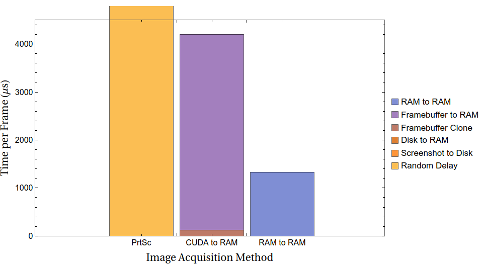
By default, the framebuffer consists of 8-bit integer values for each pixel, so we used rustacuda to call a custom CUDA kernel to convert the 8-bit integer 1600x900x3 tensor into a 32-bit floating point 1600x900x3 tensor. This is still pretty fast: 400 μs. And then, we’re ready to run the neural networks themselves.

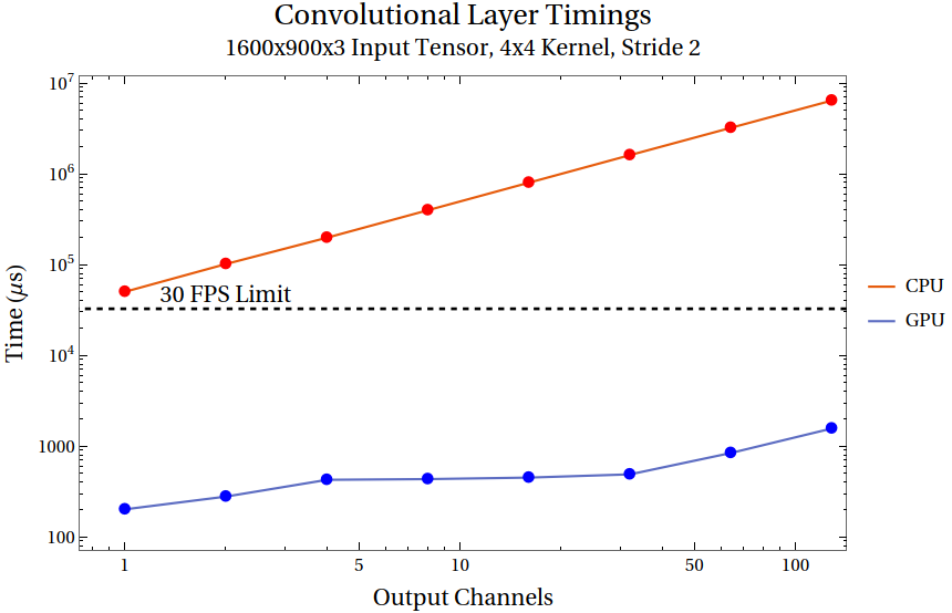
The GPU implementation of the convolutional layers showed an enormous improvement - around three orders of magnitude - over the CPU implementation. Our neural architecture ‘stack’ consisted almost entirely of convolutional layers, with one final fully-connected linear layer at the end, so all we needed to do was get a linear layer and we would be done.

cuDNN does have a full suite of convolutional layer forward and backwards activation functions, as you would expect. However, it doesn’t have a fully-connected linear layer activation…even though the fully-connected linear layer is just matrix multiplication, and is the simplest possible neural architecture. Instead, you have to use a workaround and activate a convolutional kernel whose dimensions are the same as the tensor itself, according to the official developer forums; a moderator there suggested that on the same hardware we use, this is 50% slower than the equivalent matrix multiplication would be.

Sure enough, the fully-connected layer was now our bottleneck and slowest layer by far; we discovered that the 50% number was a lower bound, and that it could get substantially worse than 50% slower, scaling with the size of the input image; for the specific dimensions we were aiming for, the linear layer ended up taking as long as all the other convolutional layers put together, effectively doubling the amount of time needed to process a frame.

Still, we only had to call that layer once, and twice a small number is still a small number. The fully-connected layer was slow, yes, but it was fast enough for our purposes, even on a full-resolution screen, to process the image and send the results to RAM with time to spare.

But it wasn’t good enough for us.

And that is where we stopped.

The Last Straw

We’ve buried the lede a bit on this post. Astute readers might have wondered how we connected and accessed these arbitrary GPU functions in proprietary libraries. Yes, the cudnn crate does indeed handle convolutional layers, and the nvfbc crate does indeed allow for framebuffer capture, and the cuda crate does indeed allow Rust to do tensor manipulation in GPU memory. All that is true. What we didn’t mention is that none of these crates were compatible with each other, and all of them are (as of 2024) nearly a decade old. The Rust cudnn crate runs against cuDNN version 3. The current version of cuDNN is 9.5. Almost every single method available in the Rust crate is deprecated, gone, or works very subtly differently in 9.5. Not to worry, the rust-cuda crate only needs CUDA 8+, while the current version is 12.6. cuDNN version 3 wants CUDA 7, of course.

You might see this list and think “No problem! Update everything to the latest major version. Surely, theres no way most major functions would be renamed or deprecated in each release…” If you think that way (as we did), you’re in for an unpleasant surprise, as we were when we got an error that simply read Unable to register an OpenGL buffer to a CUDA resource (result: 3) - NVFBC_ERR_CUDA . What does result 3 mean? What is NVFBC_ERR_CUDA? How have the error messages changed from one version to another? Hours of fruitless searching followed.

To make this work, we had to make our own Foreign Function Interface (FFI) bindings for all three crates (using cargo:rustc-link-lib= in build.rs), and then carefully make higher-level functions to access, transfer, and alter CUDA memory. It’s possible - as it always is - that this wasn’t necessary, and that there was an easy way to make all three crates talk to each other that we simply didn’t know about. But that was the whole problem. The very first thing we ever did with GPU programming was making our own interface for four separate libraries not designed to talk to each other. We didn’t know what we were doing, couldn’t find any examples of people trying to do the same thing, and didn’t know where to look

The obvious starting point was the NVIDIA documentation, but NVIDIA’s documentation is less than ideal. For instance, the developer overview for cuDNN lists, in the introduction:

NVIDIA cuDNN provides highly tuned implementations of operations arising frequently in DNN applications:

• Convolution forward and backward, including cross-correlation
• Matrix multiplication …

We looked far and wide for this matrix multiplication capability within cuDNN (matrix multiplication being equivalent to a fully-connected linear layer, the type of layer we desperately needed), and we could not find it. NVIDIA’s official “Matrix Multiplication Background User’s Guide” requires cuBLAS, not cuDNN, and the few projects we could find which used cuDNN to make convolutional layers also used cuBLAS to make linear layers.

But this still doesn’t sound too bad. We already got three crates working with each other, so why not add a fourth, and get a cuBLAS.rs to add to our cuda.rs, cudnn.rs, and nvfbc.rs? We tried. And for reasons we don’t understand, we could not get the cuBLAS foreign function calls to work in Rust, no matter how we massaged or flattened the output of the final convolutional layer. We kept getting memory errors and operation errors we couldn’t track down or identify (DGEMM parameter number 8 had an illegal value), and so rather than spend more weeks trying to eventually fix that, and rather than abandoning cuBLAS and using a solution we knew was significantly slower than ideal, we did neither, and gave up entirely.

This seems extreme, but it was inevitable based on how we approached the problem. It took months to get all the other libraries working with each other; calling a custom kernel to convert the 8-bit integers in the image framebuffer into 64-bit floating points took a long time by itself. We went as far as stepping through GPU level functions using a segfault analyzer (we actually made the segfault analyzer segfault at one point). And we - this cannot be stressed enough - had no idea what we were doing.

Conclusion

It’s hard to know what to say. ‘We gave up’ is not a particularly satisfying way to end a story, even if it happens to be true. But ‘we gave up, and didn’t bother writing about it or telling anyone what happened’ is in all ways worse. So here we are. We were tempted to write an inspiring bit on how writing about your failures is as important as writing about your successes, but that felt more like an attempt at justifying failure than anything else.

If there’s a lesson to be drawn from this, it’s to not let the perfect be the enemy of the good. We made what was the fastest program for GPU convolutional network processing of GPU-generated images that we’ve ever heard of, faster even than the Linesight program we’ve looked up to all this time. If we’d gone in merely wanting something fast, we would have been more than satisfied with this. But we weren’t going to be satisfied unless we had something optimal, and that was just a bridge too far. Don’t make the same mistake we did. It’s okay for parts of your project to be imperfect.

Because when we accept imperfection, we reduce the friction wearing down our motivation. Motivation is a finite resource. Gas in the tank, so to speak. If you choose the route full of twists and turns that requires you to stop all the time, then you are often going to run out of gas before you reach the end, no matter how much “better” that route is. Every time you choose a detour, you have to account for how much motivation that will cost. Projects that succeed, are those that budget motivation correctly.

Comment found here.

But if you do get lost along the way, if you pick the fork in the road that takes you through “Boulder Valley, no gas stations for 250 miles, follow signs for DO NOT ENTER”, the least you can do is make a map of your travels. Leave a record that the sign was, in fact, correct, and the travelers that told you the valley had only one dirt road were not in fact just trying to keep you away from the scenic vistas and sense of satisfaction. There’s a saying about how it’s the journey, and not the destination, but while we enjoyed the journey, we wish we’d actually gotten to the destination.

Series